neural networks

History

This is a paper I wrote in school - I was trying to learn about the mathematical basis of Neural Networks. It needs an update and a reformatting, but I’m proud of it for its time

Examine the role of mathematics, and more specifically, calculus and finding relative minima, used in the creation and training of Neural Networks. How can this underlying mathematics help one to understand how a Neural Network works?_

Subject Area: Mathematics
Word Count: 3632 Words
May 2019 Examination Session

Introduction

Though computers today are very powerful, we still have a lot of difficulty in our modern day lives trying to get computers to do certain tasks that humans find simple. While computers can easily do a billion calculations every second, there is no clear, algorithmic way to solve certain types of problems, such as reading a license plate in a picture, or identifying whether an animal in a picture is a dog or cat. To solve this conundrum, the idea of neural networks arose. But how are these networks created? How do they learn? How can they use mathematics to solve such a seemingly abstract problem?

These questions, along with some short research, led me to compose the following Research Question:

Examine the role of mathematics, and more specifically, calculus and finding relative minima, used in the creation and training of Neural Networks. How can this underlying mathematics help one to understand how a Neural Network works?

In this Paper, I aim to investigate the essentials of Neural Networks, and how and why they work in relation to the mathematics behind them. As I continue, I will also briefly examine how Neural Networks differ from traditional methods of computing, given that Neural Networks are clearly intended to solve different types of problems than regular algorithms. In terms of their use, Neural Networks are most efficient at solving problems with messy or unclear input data, that could not be easily solved with an algorithmic, step by step approach. A variety of areas in mathematics can be used in the analysis and creation of Neural Networks, including linear algebra and vector math, graph theory, and various statistical analyses, but arguably at the core of it all is the use of Calculus and Gradient Descent, which is used in the training of the network. This is what I will primarily explore in this paper, and I will go through it in the order in which it is relevant to a neural network’s creation. Before that is discussed, one must have a basic understanding of how the concept of a Neural Network originated, and what it entails.

To begin, let us understand where the idea of an Artificial Neural Network originates from. As the name alludes to, it relates to the Natural Neural Networks that are present in organisms, which people have been interested in for as long as they realized that they have had brains. The brain itself is very complex, being comprised of several areas dedicated to different functions. Its fundamental building block is the Neuron – a cell that takes inputs of electrical charge from its dendrites (which can number in the tens of thousands), to return a single output from its axon, which either fires, or does not fire. As opposed to traditional computing methods, which tend to be only slightly multi threaded and fast, neural networks tend to be more dependent on parallel processing and slower individual processes (Coolen, 2003). Furthermore, as opposed to traditional algorithms, Neural Networks have a degree of “training” in which the program is optimized for its specific function, as has been alluded to before (Coolen, 2003).

Conventional Computers	Biological Neural Networks
Processors	Neurons
operation speed ~ 10⁸ Hz	operation speed ~ 10² Hz
signal/noise ~ ∞	signal/noise ~ 1
signal velocity ~ 10⁸ m/sec	signal velocity ~ 1 m/sec
connections ~ 10	connections ~ 10⁴
Sequential operation	Parallel operation
Program & data	Connections, neuron thresholds
External programming	Self-programming & adaptation
Hardware failure: fatal	Robust against hardware failure
No unforeseen data	Messy, unforeseen data

Table 1: Source derived from an article on the fundamentals of the math behind neural networks (Coolen, 2003)

Structure and Building Blocks of the Neural Network

To continue, this idea of a Network of cells can be simplified into a computation method. Essentially, a neuron could be represented by a function taking in a certain number of variables, and transforming its given data to a single output variable. Putting a large number of these Neurons together results in a Neural Network, which consists of an input layer (which consists of the data put into the network), a certain number of hidden layers (the layers that do the “processing”), and an output layer (which is what outputs the network’s result) (McDonald, 2017). In essence, a neural network is just a network of functions feeding into each other to result in an output. A diagram is shown below:

An important question to be asking while examining this is why this structure results in the input it does. Why would a grouping of functions be able to figure out the character that is written by my messy handwriting? Well, while a traditional algorithm would solve a problem step by step, with the instructions that it is given, similar to a single function, Neural Networks consist of several of these functions (or what will be called nodes, neurons, or vertices), which essentially allows the problem to be reduced into different parts and chunked together. Each layer examines a specific part of the problem, and each neuron examines a specific part of its layer’s problem. However, this is just speculation, as it can be notoriously difficult to find out why a network does one thing as opposed to something else. This will be explored further when the training of networks is examined. 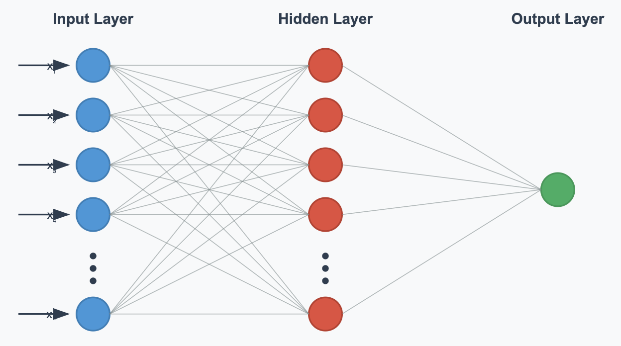Figure 2: Source derived from an article about the basic layout of a Neural Network (Khademi, 2016)

The layout of a single neuron, and the equation of a Neuron

Delving deeper into the structure of a network, one Neuron follows the diagram below:

The input layer can be represented by the vector $\vec{x}$, while the weights of the corresponding connection to the neuron in question can be represented by $\vec{w}$. The activation threshold, or other factors related to firing of the neuron are represented by $b$, which is called the bias. The formula below shows the how the output of the neuron, $v$ is calculated:

$\vec{x}\cdot \vec{w}+b=v$

In this way, stronger connections with a neuron represent higher weights for it, and a greater contribution to its input (McDonald, 2017). Bias relates to essentially increasing or decreasing the input value for a neuron by adding a number to to the dot product of the weight and value vectors (McDonald, 2017). 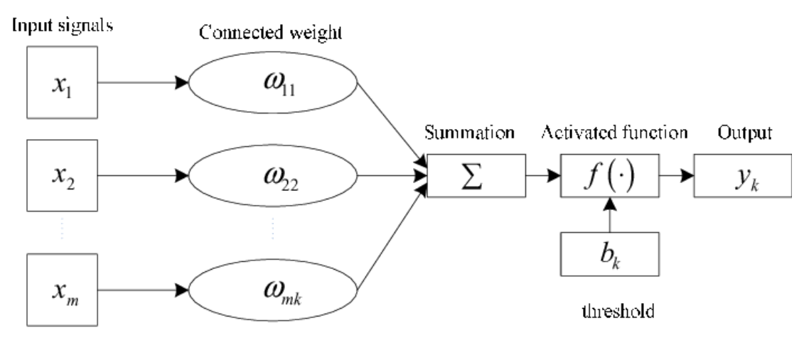Figure 3: Source derived from an article on the basic structure of a Neuron (Ying, 2014)

Transforming the output of a neuron with the Heaviside Step and Sigmoid functions

This is transformed by the function $f(v)$ to result in the final transformed output of the function, which can be many things. In a traditional neuron, the transformed output would be considered either 1 or 0 – the neuron either fires, or it doesn’t fire. This is represented by the Heaviside Step function, shown b:

The Heaviside Step function is defined by the following piece wise function:

$f(v)=\{\begin{array}{llc}1,& v>00,& v<0\end{array}$

Another possible function for $f(v)$ is the Sigmoid function, a continuous function that ranges from 0 to one. This is obviously only possible for artificial neural networks that are not only limited to 2 values. This would allow artificial neural networks to carry much more information per neuron as compared to a natural one. This function is graphed on the following page: 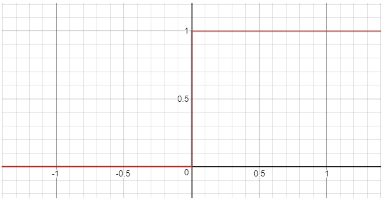Figure 4: Graphed using Desmos.com graphing tool

The Sigmoid curve is defined by the function:

$f(v)=\frac{1}{1+e^{-v}}$

Essentially, these functions represent the neuron itself, and the transformation it does to result in its transformed output. To keep all the numbers within the Network on the same degree of magnitude, the Sigmoid function is used, as it continuously maps its domain, $v|v\in \mathbb{R}$ to its range, $f(v)|f(v)\in [0,1]$. One important thing to note in detailing the Sigmoid function, and the reason why it is most commonly used as the transformation function for every Neuron, is its continuous and differentiable nature. This is important to the gradient descent step in finding the minima of the Cost Function, which will be examined soon. This concludes the basic layout of the Neural Network, how data is fed into it, and the basic structure of the nodes themselves. However, one large question remains- how do we find values for the weights and biases of each Neuron? 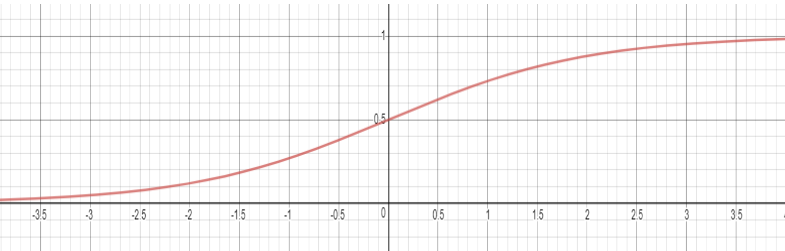Figure 5: Graphed using Desmos.com graphing tool

Training of Neural Networks with forward and back propagation and gradient descent

The answer to the previous question is simple in name, but is in fact one of the most extensive parts of creating a Neural Network – the network must be trained. This is done with a significant amount of training and test data – sample data that could be fed into the Network, for which ideal results for have already been obtained. This data is obtained from humans that have solved this problem in the way that they think is right – think of the CAPTCHA(Completely Automated Public Turing test to tell Computers and Humans Apart) boxes that one must fill out to prove that they are not a robot on websites. These generally have 1 box for which they have data, and one for which they need to get data. By verifying the result using one of them and using the other as new data, data that can be used to train these networks is crowd sourced.

Forward Propagation

The first step in the process is fairly simple. The Neural Network is initialized with completely random values for these weights and biases, which will definitely result in random values. Data is then inputted into the input layer of the neural network, like it would be fed into one normally. This is called forward propagation, as the training input data propagates forward through the layers of neurons until it reaches the end of the network – the output layer.

The Cost Function

To continue, it becomes necessary to find a way to quantify how much the weights and biases must be changed. To do this, a function that measures how incorrect the network is can be created – something called the cost function. It will take in the weights and biases of the network as inputs to the function, and return a single value that can quantify the error of the function in relation to this specific training sample. This is done by summing the squared difference between the actual and expected values of the output layer, for a single training sample. A general Cost Function is shown below:

$C(w_1,w_2,...,w_n,b_1,b_2,...,b_m)={\sum }_{i=t-s}^t(T_i-f(v_i){)}^2$

Where $w_1,w_2,...,w_n$ represent the $n$ weights of the network, $b_1,b_2,...,b_m$ represent the $m$ biases of the graph, $v_{t-s},v_{t-s+1},...,v_t$ represent the $s$ neurons of the output layer, and $T_{t-s},T_{t-s+1},...,T_t$ represent the $s$ corresponding pieces of training data expected values for this particular training data sample.

To be clear, though there are no actual mentions of $w_1,w_2,...,w_n$ and $b_1,b_2,...,b_m$ in the right hand side of the equation, these are still the only variables for this function, as any $f(v_i)$ in the final layer (for $t-s⩽i⩽t$) can be seen as the linear combination of the transformed outputs of the previous layers neurons weights, the previous neuron’s transformed outputs, $f(v_i)$ (for $i<t-s$), and the biases of the neurons in the current layer. In this way, the cost function can be expanded as necessary, thereby backwards propagating through the network from the output layer to previous layers as necessary. This is not specifically back propagation yet however, as back propagation involves the changing of the weights and biases through the minimization of the Cost Function.

Gradient Descent and Back Propagation

Another important note that will be crucial in having a more holistic understanding of training neural networks is the nature of the training data that is used. The training data expected values that are used in this general Cost Function all come from what humans determine should be the expected value for a given sample of training input data. For example, If the training input data is a 16 x 16 bitmap of a handwritten character, the training data expected values would come from a human looking at this bitmap and determining that the character is an “e” for example. As a result of this, back propagation and gradient descent that will be done with this Cost Function will pertain to one training sample. The complete training of the network consists of repeating the processes of gradient descent and back propagation for different Cost Functions, each of which are based upon an individual training data sample in a complete set of training data.

Visuals can be crucial to have a better intuitive understanding of how back propagation and gradient descent works. To do this, I will graph a sample simplified Cost Function in 3 Dimensions. This sample Cost Function will have two inputs and one output, as shown below:

As can be seen, the function itself is continuous and differentiable, as it is composed of repeated linear combinations of the Sigmoid function, which itself is continuous and differentiable, the connection weights and the neuron biases In the end, the function itself is continuous and differentiable for all inputs $x,y\in {\mathbb{R}}^2$. Considering that any possible combination of weights and biases exist on the input plane of this graph, I know that the initial random values chosen for the weights and biases are somewhere on this input plane, and it is also likely that they have a high cost. The problem of training this network then reduces to finding a way to reduce this cost to as much as possible – which can be done by finding a relative minimum of the Cost Function. As can be seen in the graph above, even though a relatively simple Cost Function in 3 Dimensions can have many relative minima, it would be difficult to find an absolute minimum. This reduces the task of training the neural network to finding a relative minimum of the cost function, which is considered “good enough” by most (this will be further explored in the training data section). This will be accomplished through gradient descent. As I continue, I will augment this problem back to an arbitrary number of input dimensions for more applicable equations without loss of generality.

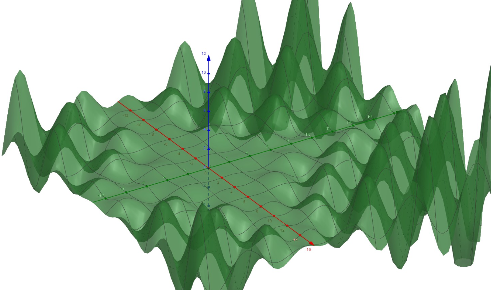Figure 6: Graphed using the Geogebra.org 3D graphing tool

Furthermore, to make the notation more simple in the following sections more simple, I will also introduce a vector form of the Cost Function that will be significantly less verbose. This function is shown below:

$C(\overrightarrow{wb})=|\vec{T}-\overrightarrow{x_f}{|}^2$

Where $\overrightarrow{wb}$ represents the vector of weights and biases (represented by $w_1,w_2,...,w_n$ and $b_1,b_2,...,b_m$ in the previous equation), $\overrightarrow{x_f}$ represents the vector of output values from the final output layer of the network (represented by $f(v_i)$ for specific values of $i$ in the previous equation) and $\vec{T}$ represents the vector of corresponding pieces of training data expected values (represented by $T_{t-s},T_{t-s+1},...,T_t$ in the previous equation).

Gradient descent is simply a method to move towards an approximation of a relative minimum of the Cost Function by using the gradient of the function. Considering that the gradient of the Cost function at the current combination of weights and biases of the graph would give the direction in which the cost would increase most quickly, we use the negative gradient of the Cost Function at this point, to find the direction in which the weights and biases should move to decrease the cost most quickly, moving towards a relative minimum of the graph. To accomplish the aforementioned task in mathematical terms, we can use the recurrence relation below:

${\overrightarrow{wb}}_{n+1}={\overrightarrow{wb}}_n-\nabla C{|}_{{\overrightarrow{wb}}_n}\cdot s$

Where ${\overrightarrow{wb}}_n$ represents the $n$th iteration of the weights and biases vector (so ${\overrightarrow{wb}}_0$ is the first iteration, consisting of the random weights and biases that initialize the network). $s$ represents an arbitrary step size that can be decreased to increase the precision of the approximation, but make the algorithm slower, while increasing $s$ will decrease the precision of the approximation, while making the algorithm faster.

In reference to a specific weight or bias and how much it should be changed, we can use the specific partial derivative respective to that weight or bias. This is shown in the recurrence relation below, which can be seen as a specific part of the previous recurrence relation:

$w{b}_{i,n+1}=w{b}_{i,n+1}-\frac{\partial C}{\partial w{b}_{i,n}}\cdot s$

Where $w{b}_{i,n}$ represents the $n$th iteration of the $i$th weight or bias. We use the partial derivative of $C$ with respect to the weight or bias $w{b}_{i,n}$ as to determine how much this specific variable affects the cost function, all other variables must be treated as constants, which is the definition of the partial derivative.

This is the specific equation used in the back propagation algorithm. It is also important to recall that the cost function is expanded as need be, allowing for the partial derivatives of $C$ with respect to a specific weight or bias $w{b}_{i,n}$ to be found. To do this, the chain rule can be applied as such:

$\frac{\partial C}{\partial w{b}_{i,n}}=\frac{\partial C}{\partial x_{f,i}}\cdot \frac{\partial x_{f,i}}{\partial x_{f-1,i}}\cdot \frac{\partial x_{f-1,i}}{\partial x_{f-2,i}}\cdot \cdots \cdot \frac{\partial x_{r,i}}{\partial w{b}_{i,n}}$

Where $x_{f,i}$ represents the transformed output of the $i$th neuron in row $f$. Essentially, with this, successive partial derivatives are taken to find the relationship between a differential change in one neuron, to the neuron behind it, all the way until the neuron for which that specific weight or bias is attached to is reached. When this is reached, the partial derivative of the transformed output of that neuron in relation to that weight or bias can be taken, giving the end result with the chain rule.

As this algorithm is iterated, the weights and biases will be adjusted quickly at first, and more slowly as a relative minimum of the graph is approached. This is due to the magnitude of the partial derivatives and gradient vector itself decreasing as a relative minimum is approached, as the changes that must be made to the weights and biases become smaller as a relative minimum is approached. After a relative minimum is reached, this process of forward propagation, gradient descent, and back propagation are repeated for different Cost functions from different training data samples. Finally, after the training data has been run through, the time comes to test this trained neural network.

Testing a Neural Network with Test Data

Even with a Neural Network that has been trained with thousands of pieces of sample data, we cannot be sure if it works with real world data unless it is tested. To test it, test data is inputted into the Network, which is similar to training data in that expected values for it have been obtained, but this data itself is completely new to the network – which has never trained for this specific sample. By running this data through the neural network, we can test its ability to remain accurate in a real world setting for which it has to extrapolate expected values for data it has never seen. In a sense, this can be thought of as a check step for the Neural Network.

In my initial understanding of testing data, I did not understand the point of it, but I soon realized that the necessary of testing data all comes back to the idea of finding a minimum of the Cost Function with Gradient Descent. To better examine this, I will go down to a sample Cost Function with a one variable input and output, shown below:

In this figure, it can be seen that there exist several relative minimums to the cost function, and with the way that Gradient Descent works, slowing down when any relative minimum is reached, the back propagation algorithm could end when the first relative minimum, which still has a high cost, is reached. So even if the back propagation completes with a certain data sample, it is still not certain whether the network was effectively able to “learn” from this sample by changing its weights and biases in the most efficient way. 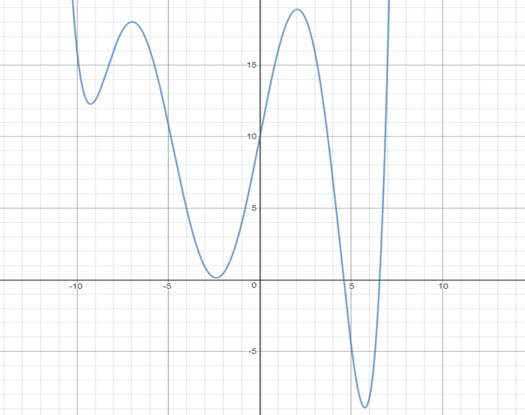Figure 7: Graphed using Desmos.com graphing tool

There is also the problem of over fitting or under fitting the data, in which a network either over fits or under fits its training data, resulting in it not being a good model to test data from the real world. This can be shown in the figure below:

If a network is trained to be overly reliant on its training data, then it will not function well with real world data, with a lot of introduced noise, but if it under fitted, the network will not be able to make good conclusions from the data it gets because it never “learned” anything. To ensure this, the sample data set must be an appropriate size and diversity for the training of the network. 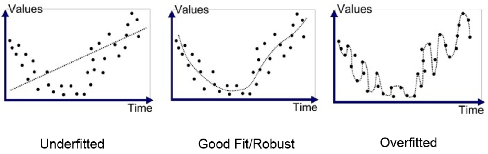Figure 8: Source derived from a paper on over/underfitting in machine learning (Bhande, 2018)

This is why testing a neural network is important, but the process itself is a fairly short checking step. Test data is fed into the network, and the number of correct samples over the total samples results in the accuracy. If a neural network is accurate, then it can go on into real world use, but if it is not, there are a variety of other steps that can be taken – go back and retrain the network with new training data, change the layout of the network, or several other possible options.

Conclusion

In this paper, I aimed to investigate the concept of a Neural Network, and the underlying math behind it, with the following Research Question:

Examine the role of mathematics, and more specifically, calculus and finding relative minima, used in the creation and training of Neural Networks. How can this underlying mathematics help one to understand how a Neural Network works?

Through this investigation, I learned that though there is a variety of mathematics that can be used in the creation and analysis of neural networks, such as vector math and various statistical analyses. In terms of vector math/linear algebra, it is not necessarily used in a specific part of the process, but can be used in the simplification of equations surrounding the neural network and its notation – for example, the initial cost function compared to its vector form that I later created. Also, though statistical analyses were only touched on very briefly in this paper, they can also be used to analyze a network. Though these aforementioned areas of mathematics are important in creating and analyzing neural networks, the idea of finding relative minima of a function lies at the heart of it all, in the training of the neural network. This is the part in creating a neural network that actually relies on it “learning” and fitting itself to a give a certain output, when given a specific form of input data through the back propagation algorithm. As this is the case, the consequences of using the gradient descent to find the relative minima of weights and biases show up in other places in the analysis of the neural network, such as the testing phase – which revolves around the idea that gradient descent is not able to find the best relative minimum sometimes. This also reveals noteworthy thing about neural networks that is key to understanding them – training them can result in many different final results, due to the presence of many possible relative minima of the Cost Function.

References

Bhande, A. (2018, March 11). [Underfitting, overfitting, and good fit] [Chart]. Retrieved from https://medium.com/greyatom/what-is-underfitting-and-overfitting-in-machine-learning-and-how-to-deal-with-it-6803a989c76

Coolen, A. C.C. (2003). A beginner’s guide to the mathematics of neural networks. In A. C.C. Coolen (Author), Concepts for neural networks. Retrieved from CiteseerX database.

Khademi, F. (2016, May). Structure of the artificial neural network model [Illustration]. Retrieved from https://www.researchgate.net/figure/shows-the-training-state-for-the-artificial-neural-network-model-As-it-is-illustrated-in_fig1_305432476?_sg=sMUzOsV8JWgcUbpR6i50hMd-8Q0V1VnnHYxo8VkUnFH7wLrEKeTTmQc7t_UChe-VMizPyFCMbl50XhcLEefbF_DdqD9PxrNmZTvunEjoHg

McDonald, C. (2017, December 21). Machine learning fundamentals (II): Neural networks [Formal article]. Retrieved January 11, 2019, from Towards Data Science website: https://towardsdatascience.com/machine-learning-fundamentals-ii-neural-networks-f1e7b2cb3eef

Ying, Y. (2014, November). The unit of artificial neuron model the work process of neural network [Illustration]. Retrieved from https://www.researchgate.net/figure/The-Unit-of-Artificial-Neuron-Model-The-work-process-of-neural-network-can-be-summarized_fig1_301410002